Assigning Geometric Properties#
Geometric properties refer to the physical sizes of the pores and throats, such as pore diameter and throat lengths. The values are essential to the pore network modeling enterprize since they control all the transport and percolation behavior of the network. Unlike phase properties which can be normalized for, geometric properties define the network even more than topological properties like connectivity.
Geometric properties can be calculated by various means, ranging from assigning random values to pores, to extracting values from tomographic images. OpenPNM provides a library of functions, or ‘pore-scale models’ which can calculate these geometric properties automatically. This tutorial will cover the following subjects:
Manually Calculating Pore and Throat Properties (⚠ Not Recommended!)
Using Pore-scale Models from the Library
Overview of the Dependency Handler
Using Predefined Collections of Models
Defining Heterogeneous Domains (by Applying Models to Specific Locations)
Customizing Models (by Overwriting Them or Their Arguments)
Writing and Using Custom Models
import numpy as np
import matplotlib.pyplot as plt
import openpnm as op
import scipy.stats as spst
op.visualization.set_mpl_style()
Let’s start by creating a blank Cubic network. As we can see by printing it, there are only coordinates, connections, and some labels, but no geometric properties:
np.random.seed(0)
pn = op.network.Cubic([20, 20, 20], spacing=5e-5)
print(pn)
══════════════════════════════════════════════════════════════════════════════
net : <openpnm.network.Cubic at 0x7f51a7da3110>
――――――――――――――――――――――――――――――――――――――――――――――――――――――――――――――――――――――――――――――
  #  Properties                                                   Valid Values
――――――――――――――――――――――――――――――――――――――――――――――――――――――――――――――――――――――――――――――
  2  pore.coords                                                   8000 / 8000
  3  throat.conns                                                22800 / 22800
――――――――――――――――――――――――――――――――――――――――――――――――――――――――――――――――――――――――――――――
  #  Labels                                                 Assigned Locations
――――――――――――――――――――――――――――――――――――――――――――――――――――――――――――――――――――――――――――――
  2  pore.xmin                                                             400
  3  pore.xmax                                                             400
  4  pore.ymin                                                             400
  5  pore.ymax                                                             400
  6  pore.zmin                                                             400
  7  pore.zmax                                                             400
  8  pore.surface                                                         2168
  9  throat.surface                                                       4332
 10  pore.left                                                             400
 11  pore.right                                                            400
 12  pore.front                                                            400
 13  pore.back                                                             400
 14  pore.bottom                                                           400
 15  pore.top                                                              400
――――――――――――――――――――――――――――――――――――――――――――――――――――――――――――――――――――――――――――――
Attention
Changed in V3
In OpenPNM V3 we have removed the concept of Geometry and Physics objects, in favor of placing all the properties on the Network and Phase objects instead.
To add geometrical properties to a network, we have a few different options. Each will be explored below:
Manually Calculating Properties#
Warning
Manual Calculation is Not Recommended
This is not the preferred way to do things, but does illustrate the processes very well. The preferred way is using pore-scale models, which allow for the automatic regeneration of dependent properties when something changes.
Let’s start by adding pore and throat size distributions. There are a few different ways to do this, and we’ll explore each one to be thorough.
Adding pore and throat sizes from scipy.stats distributions#
Scipy’s stats module has a lot of statistical distributions defined. Let’s generate pore and throat sizes using some of these. First, let’s use a normal distribution to generate pore sizes within the range ~1 to 50 um:
np.random.seed(0)
psd = spst.norm.rvs(loc=25, scale=6, size=pn.Np)
plt.hist(psd, edgecolor='k')
plt.xlim([0, 50]);

The above distribution looks good, let’s just make absolutely sure that our distribution is not so wide that it has negative numbers or values greater than 50 um:
print(psd.min())
print(psd.max())
2.5593961722893255
47.80996128980269
Now we’ll convert these values to SI and assign to the network:
pn['pore.diameter'] = psd*1e-6 # um to m
Next we need to define throat diameters. We can do this in the same way, but let’s use a different distribution. Note that this approach is not recommended because as we’ll see it results in throats that are larger than the two pores they are connected two. We’ll fix this in the following section:
np.random.seed(0)
tsd = spst.weibull_min.rvs(c=1.5, loc=.5, scale=7.5, size=pn.Nt)
plt.hist(tsd, edgecolor='k')
plt.xlim([0, 50]);

Again, let’s inspect the high and low values:
print(tsd.min())
print(tsd.max())
0.5130345457395142
36.96861960231873
So we can see that we have throats as small as 500 nm, and as large as 37 um. These can be assigned to the network as well:
pn['throat.diameter'] = tsd*1e-6 # um to m
The problem with this approach is that both pore and throat sizes were just assigned to random locations, rather than putting small throats between small pores and vice-versa. When throats are larger than the pores they connect it can cause problems or strangeness in the results since we generally assume a throat is a constriction between two pores. Let’s count how many are problematic.
hits = np.any(pn['pore.diameter'][pn.conns].T < pn['throat.diameter'], axis=0)
hits.sum()
np.int64(564)
Tip
Indexing pore properties by conns: Using the conns array to index into a pore property returns an Nt-by-2 array with the properties of the pores on the end of a throat in each column. For instance, see the diameter of the pore on each end of a throat, use pn['pore.diameter'][pn.conns]. This approach is very powerful. If you ever feel tempted to use a for-loop to scan over each pore, then inspect the properties of the neighboring throats, consider instead if you can “loop” over the throats then interrogate each pore. If yes, then you can use this conns-indexing trick.
There are two safer ways to assign pore and throat sizes, to ensure that throats are smaller than the pores they connected. The first is to proceed as above by assigning pore sizes randomly, then assigning throats to be the as small (or smaller) as the smallest pore it is connected to. This can be done using some numpy functions as follows:
tsd = np.amin(pn['pore.diameter'][pn.conns], axis=1)
plt.hist(tsd, edgecolor='k', density=True, alpha=0.5)
plt.hist(pn['pore.diameter'], edgecolor='k', density=True, alpha=0.5)
plt.xlim([0, 50e-6]);

We can see from the above plot that the throat sizes are similar to the pore sizes, which is expected since they are taken from the pore sizes values. However, we can also see a small shift to the left, which is also expected given that the throats always take on the size of the smaller pore, creating a bias towards smaller sizes.
It may also be desirable to force the throats to be smaller than the two neighboring pores by some factor:
pn['throat.diameter'] = tsd*0.5
plt.hist(pn['throat.diameter'], edgecolor='k', density=True, alpha=0.5)
plt.hist(pn['pore.diameter'], edgecolor='k', density=True, alpha=0.5)
plt.xlim([0, 50e-6]);

One downside of the above approach is that you no longer have control over the shape and distribution of the throat sizes. This can be solved by applying the same approach just described but to random seeds instead of actual sizes. Then the random seeds can be put into a cumulative density function to compute the corresponding size. This is demonstrated below:
lo, hi = 0.01, 0.99
pn['pore.seed'] = np.random.rand(pn.Np)*(hi - lo) + lo
Tip
Setting the lo and hi values of the seeds prevents values that lie far out in the tail of a distribution from occurring which can lead to overly large pores or throats.
The ppf function, or point probability function returns the value of a cumulative distribution at the given probability, so the seed values computed above can be related to size values using:
import scipy.stats as spst
psd = spst.norm.ppf(loc=25, scale=6, q=pn['pore.seed'])
pn['pore.diameter'] = psd*1e-6
plt.hist(pn['pore.diameter'], edgecolor='k')
plt.xlim([0, 50e-6]);

Now we can find the throat seed values as the minimum pore seed value of the two neighboring pores:
pn['throat.seed'] = np.amin(pn['pore.seed'][pn.conns], axis=1)
And then we can use these seed values in the ppf function of the desired distribution. So long as the distribution does not create larger values than the distribution used to compute pore sizes, then the throat sizes will always be smaller.
tsd = spst.norm.ppf(loc=25, scale=6, q=pn['throat.seed'])
pn['throat.diameter'] = tsd*1e-6
plt.hist(pn['throat.diameter'], edgecolor='k', density=True, alpha=0.5)
plt.hist(pn['pore.diameter'], edgecolor='k', density=True, alpha=0.5)
plt.xlim([0, 50e-6]);

Once the pore and throat diameters are specified, the next step is to define any dependent properties of interest, such as pore volume or throat length. These additional calculations tend to require that we assume a shape for the pores and throats. It is not mandatory to use spheres and cylinders, though this is a common choice. We could also work with cubic pores and cuboid throats, which occupy a large volume fraction for instance. The choice of cubic shapes also happens to make the calculations much easier, for reasons explored below, so in this tutorial we’ll assume cubic shapes. Let’s calculate the throat length, and pore surface area, since each of these illustrate very important concepts regarding the use of vectorized calculations.
Computing throat length#
Throat length is the pore-to-pore spacing, less the radius of each pore. This can be found without the need for a for-loop using the following vectorization trick:
R1, R2 = (pn['pore.diameter'][pn.conns]/2).T
L_total = np.sqrt(np.sum(np.diff(pn.coords[pn.conns], axis=1).squeeze()**2, axis=1))
Lt = L_total - R1 - R2
print(L_total)
[5.e-05 5.e-05 5.e-05 ... 5.e-05 5.e-05 5.e-05]
The above cell contains 3 complicated but powerful steps:
The radii of the pores on each end of each throat are retrieved.
R1andR2contain duplicates since each pore has numerous throats, so they appear once for each throat. This fact is used in step 3.The pore-to-pore distance is found by retrieving the coordinates of each pore, in the same was as was done for the radii. The Euclidean distance between each pair of pores is then computed by finding their difference (
np.diff), squaring it, summing it (np.sum), then taking the square root (np.sqrt) of each. Theaxisargument is used throughout to tell numpy which way to apply the operation. This line is an example of how you must learn a mini-language to use numpy effectively.The length of each throat is found as the spacing between pores, less the radii of the pore on each end. This is where the duplicate values in
R1andR2are necessary, since the radii of pore i must be subtracted from length of each of its neighboring throats.
The main take-home message here is that throat properties can be computed in a vectorized way, even if some pore-properties are required. This avoids the use of a for-loop to scan through a list of throats followed by a nested for-loop to scan through each neighboring pore.
Computing pore surface areas#
The pore surface area is the total area of the cubic pore body, less the cross-sectional area of each neighboring throat. This can also be found without a for-loop, but requires knowing some deeper numpy functionality, known as unbuffered in-place operations:
At = pn['throat.diameter']**2
SAp = (pn['pore.diameter']**2)*6
np.subtract.at(SAp, pn.conns[:, 0], At)
np.subtract.at(SAp, pn.conns[:, 1], At)
print(SAp)
[9.08485305e-10 5.68134509e-09 2.33947201e-09 ... 6.57211706e-10
 1.92152447e-09 1.72429278e-09]
The above cell contains 2 lines of importance, which each do almost the same thing:
The first line subtracts the throat cross-sectional area from each pore listed in the first column of the
pn.connsarray. Since a given pore is connected to potentially many throats, the subtraction must be done usingnp.substract.atwhich is a special version of the subtract function that subtracts every value inAtfrom the locations inSApindicated bypn.conn[:, 0], and it does so in a cumulative fashion. Thus if pore i appears inpn.conns[:, 0]more than once, then more than one value ofAtis removed. The operation is performed in-place so that no array is returned.Recall that
pn.connscontains only the upper-triangular entries of the adjacency matrix, so this process only gets half of the connections. This means that the pore connections found inpn.conns[:, 1]must also be analyzed.
Using Pore-scale Models from the Library#
The above section is quite lengthy, but lays bare the process of computing geometric properties of a network for illustration purposes. In this section we’ll utilize OpenPNM’s library of ‘pore-scale’ models to get the same job done much more easily. Start by generating a fresh network:
np.random.seed(0)
pn = op.network.Cubic([20, 20, 20], spacing=5e-5)
First let’s assign a random number to each pore, but instead of using np.random.rand directly, we’ll use a pore-scale model:
f = op.models.geometry.pore_seed.random
pn.add_model(propname='pore.seed',
             model=f,
             seed=None,  # Seed value provided to numpy's random number generator.
             num_range=[0.01, 0.99],)
Note
Where do models go?
We’ll look more closely at models later in this tutorial, but it’s worth pointing out that the add_model method collects all the arguments provided and stores them in the models attribute of the object. Later, when regenerate_models is called, it looks into the models attribute and fetches the model (f) and the given arguments, calls the function, collects the returned result, and stores them in pn[propname]. You can see a list of models applied to the object with print(pn.models).
Let’s have each throat inherit the minimum seed value found in each of its neighboring pores, for which OpenPNM provides a model:
f = op.models.geometry.throat_seed.from_neighbor_pores
pn.add_model(propname='throat.seed',
             model=f,
             prop='pore.seed',
             mode='min')
Tip
Using shift-tab to see the docstring
In the above two code blocks the models were assigned to f first, then f was passed to the model argument. This is helpful for two reasons. (1) It helps keep the line length below Python’s preferred limit of 78 characters, and (2) it makes it possible to see the docstring of the model by putting the cursor at the end of the first line and hitting shift-tab. Seeing the docstring really helps to understand what a model does and what arguments are required.
Now we can compute pore and throat sizes from distributions, which are also provided as OpenPNM models:
f = op.models.geometry.pore_size.normal
pn.add_model(propname='pore.diameter',
             model=f,
             scale=1e-5,
             loc=2.5e-5,
             seeds='pore.seed')
plt.hist(pn['pore.diameter'], edgecolor='k');

And similarly we fetch a model for the throat sizes as well:
f = op.models.geometry.throat_size.normal
pn.add_model(propname='throat.diameter',
             model=f,
             scale=1e-5,
             loc=2.5e-5)
plt.hist(pn['pore.diameter'], edgecolor='k', density=True, alpha=0.5)
plt.hist(pn['throat.diameter'], edgecolor='k', density=True, alpha=0.5);

Now that we have pore and throat sizes, we can compute their volumes (and other properties). The volume will depend on the shape of the pores and throats. In OpenPNM we do not explicitly track such shapes. Instead we offer several models that calculate the property of interest for a given shape. This is illustrated below:
f = op.models.geometry.throat_length.spheres_and_cylinders
pn.add_model(propname='throat.length',
             model=f)
f1 = op.models.geometry.pore_volume.sphere
pn.add_model(propname='pore.volume',
             model=f1)
f2 = op.models.geometry.throat_volume.cylinder
pn.add_model(propname='throat.volume',
             model=f2)
Warning
Spherical pores overlap with their throats
A spherical pore will always have a region of overlap with its connected throats. The volume of this region will be double counted if an extra step is not taken.
f = op.models.geometry.throat_length.spheres_and_cylinders
pn.add_model(propname='throat.length',
             model=f)
f1 = op.models.geometry.pore_volume.sphere
pn.add_model(propname='pore.volume',
             model=f1)
f2 = op.models.geometry.throat_volume.cylinder
pn.add_model(propname='throat.total_volume',
             model=f2)
f3 = op.models.geometry.throat_volume.lens
pn.add_model(propname='throat.lens_volume',
             model=f3)
f4 = op.models.misc.difference
pn.add_model(propname='throat.volume',
             model=f4,
             props=['throat.total_volume', 'throat.lens_volume'])
We can inspect some of these values to make sure they are making sense:
print("Volumes of full throats:", pn['throat.total_volume'][:3])
print("Volumes of lenses:", pn['throat.lens_volume'][:3])
print("Actual throat volumes:", pn['throat.volume'][:3])
Volumes of full throats: [2.27203214e-14 2.58686910e-14 2.44028684e-14]
Volumes of lenses: [6.92245838e-15 8.40091924e-15 7.59556144e-15]
Actual throat volumes: [1.57978631e-14 1.74677718e-14 1.68073070e-14]
Using Predefined Collections of Models#
The process of selecting all the correct models from the models library can be tedious and error prone. In OpenPNM V3 we have introduced the concept of model collections, which are predefined dictionaries of models that form a complete and correct geometry. For instance, there is a collection called spheres_and_cylinders, which contains all the needed models to describe this geometry.
These collections are found under openpnm.models.collections, and their use is outlined below:
pn = op.network.Cubic(shape=[20, 20, 20], spacing=5e-5)
The models collection is fetched as follows:
from pprint import pprint
mods = op.models.collections.geometry.spheres_and_cylinders
pprint(mods)
{'pore.diameter': {'model': <function product at 0x7f518cd67ce0>,
                   'props': ['pore.max_size', 'pore.seed']},
 'pore.max_size': {'iters': 10,
                   'model': <function largest_sphere at 0x7f518aa14a40>},
 'pore.seed': {'element': 'pore',
               'model': <function random at 0x7f518cd674c0>,
               'num_range': [0.2, 0.7],
               'seed': None},
 'pore.volume': {'model': <function sphere at 0x7f518aa15080>,
                 'pore_diameter': 'pore.diameter'},
 'throat.cross_sectional_area': {'model': <function cylinder at 0x7f518aa15b20>,
                                 'throat_diameter': 'throat.diameter'},
 'throat.diameter': {'factor': 0.5,
                     'model': <function scaled at 0x7f518cd67d80>,
                     'prop': 'throat.max_size'},
 'throat.diffusive_size_factors': {'model': <function spheres_and_cylinders at 0x7f518cd66f20>,
                                   'pore_diameter': 'pore.diameter',
                                   'throat_diameter': 'throat.diameter'},
 'throat.hydraulic_size_factors': {'model': <function spheres_and_cylinders at 0x7f518aa17ec0>,
                                   'pore_diameter': 'pore.diameter',
                                   'throat_diameter': 'throat.diameter'},
 'throat.length': {'model': <function spheres_and_cylinders at 0x7f518aa16840>,
                   'pore_diameter': 'pore.diameter',
                   'throat_diameter': 'throat.diameter'},
 'throat.lens_volume': {'model': <function lens at 0x7f518aa17b00>,
                        'pore_diameter': 'pore.diameter',
                        'throat_diameter': 'throat.diameter'},
 'throat.max_size': {'mode': 'min',
                     'model': <function from_neighbor_pores at 0x7f518cd67ec0>,
                     'prop': 'pore.diameter'},
 'throat.total_volume': {'model': <function cylinder at 0x7f518aa17880>,
                         'throat_diameter': 'throat.diameter',
                         'throat_length': 'throat.length'},
 'throat.volume': {'model': <function difference at 0x7f518cd67920>,
                   'props': ['throat.total_volume', 'throat.lens_volume']}}
The print-out of the dictionary is not very nice, but it can be seen that the keys are the model names, and the values are the model itself and the various arguments for the model. This dictionary can be added to the network using the add_models_collection method as follows:
pn.add_model_collection(mods)
pn.regenerate_models()
print(pn)
══════════════════════════════════════════════════════════════════════════════
net : <openpnm.network.Cubic at 0x7f518865a8a0>
――――――――――――――――――――――――――――――――――――――――――――――――――――――――――――――――――――――――――――――
  #  Properties                                                   Valid Values
――――――――――――――――――――――――――――――――――――――――――――――――――――――――――――――――――――――――――――――
  2  pore.coords                                                   8000 / 8000
  3  throat.conns                                                22800 / 22800
  4  pore.coordination_number                                      8000 / 8000
  5  pore.max_size                                                 8000 / 8000
  6  throat.spacing                                              22800 / 22800
  7  pore.seed                                                     8000 / 8000
  8  pore.diameter                                                 8000 / 8000
  9  throat.max_size                                             22800 / 22800
 10  throat.diameter                                             22800 / 22800
 11  throat.cross_sectional_area                                 22800 / 22800
 12  throat.hydraulic_size_factors                               22800 / 22800
 13  throat.diffusive_size_factors                               22800 / 22800
 14  throat.lens_volume                                          22800 / 22800
 15  throat.length                                               22800 / 22800
 16  throat.total_volume                                         22800 / 22800
 17  throat.volume                                               22800 / 22800
 18  pore.volume                                                   8000 / 8000
――――――――――――――――――――――――――――――――――――――――――――――――――――――――――――――――――――――――――――――
  #  Labels                                                 Assigned Locations
――――――――――――――――――――――――――――――――――――――――――――――――――――――――――――――――――――――――――――――
  2  pore.xmin                                                             400
  3  pore.xmax                                                             400
  4  pore.ymin                                                             400
  5  pore.ymax                                                             400
  6  pore.zmin                                                             400
  7  pore.zmax                                                             400
  8  pore.surface                                                         2168
  9  throat.surface                                                       4332
 10  pore.left                                                             400
 11  pore.right                                                            400
 12  pore.front                                                            400
 13  pore.back                                                             400
 14  pore.bottom                                                           400
 15  pore.top                                                              400
――――――――――――――――――――――――――――――――――――――――――――――――――――――――――――――――――――――――――――――
Customizing Models by Overwriting Them or Their Arguments#
The pre-written models and collections included with OpenPNM are helpful, but you’ll almost always want to adjust some of the models to suit a specific application. This can be done by either altering the arguments of existing models, or by overwriting them all together.
Let’s first look at replacing a model with one of our choice. The spheres_and_cylinders collection uses a random distribution of pore sizes, bounded between 0 and the distance to the nearest neighbor. This can be inspected by printing the specific model as follows:
print(pn.models['pore.diameter@all'])
――――――――――――――――――――――――――――――――――――――――――――――――――――――――――――――――――――――――――――――
Property Name             Parameter                 Value
――――――――――――――――――――――――――――――――――――――――――――――――――――――――――――――――――――――――――――――
pore.diameter             model:                    product
                          props:                    ['pore.max_size', 'pore.seed']
                          regeneration mode:        deferred
――――――――――――――――――――――――――――――――――――――――――――――――――――――――――――――――――――――――――――――
Note
The @ Notation
The '@all' that has been added to the model name is new in Version 3 and means that this model should be applied to pore that have the label 'pore.dall'. This will be explained in detail in the next tutorial.
Let’s replace this with a normal distribution. This can be done with the add_model method as before.
f = op.models.geometry.pore_size.normal
pn.add_model(propname='pore.diameter',
             model=f,
             scale=1e-5,
             loc=2.5e-5,
             seeds='pore.seed')
Now print the model again to ensure it was updated:
print(pn.models['pore.diameter@all'])
――――――――――――――――――――――――――――――――――――――――――――――――――――――――――――――――――――――――――――――
Property Name             Parameter                 Value
――――――――――――――――――――――――――――――――――――――――――――――――――――――――――――――――――――――――――――――
pore.diameter             model:                    normal
                          scale:                    1e-05
                          loc:                      2.5e-05
                          seeds:                    pore.seed
                          regeneration mode:        normal
――――――――――――――――――――――――――――――――――――――――――――――――――――――――――――――――――――――――――――――
And let’s inspect the values:
plt.hist(pn['pore.diameter'], edgecolor='k');

This distribution is quite truncated, due to the 'pore.seed' values that were used. Let’s reach into that model and change this. First print the model:
print(pn.models['pore.seed@all'])
――――――――――――――――――――――――――――――――――――――――――――――――――――――――――――――――――――――――――――――
Property Name             Parameter                 Value
――――――――――――――――――――――――――――――――――――――――――――――――――――――――――――――――――――――――――――――
pore.seed                 model:                    random
                          element:                  pore
                          num_range:                [0.2, 0.7]
                          seed:                     None
                          regeneration mode:        deferred
――――――――――――――――――――――――――――――――――――――――――――――――――――――――――――――――――――――――――――――
We can see that the num_range argument is quite constrained, so let’s change it. Each model is itself a dictionary, so we can overwrite as follows:
pn.models['pore.seed@all']['num_range'] = [0.01, 0.99]
pn.regenerate_models()
plt.hist(pn['pore.diameter'], edgecolor='k');

Introduction to the Dependency Handler#
Pore-scale models clearly make life easier since you don’t have to produce the complex numpy functions by hand each time, but this is not even their best feature! The main benefit of pore-scale models is that they can be recomputed automatically. For instance, if we re-run the 'pore.seed' model, then all the other models that depend on 'pore.seed' will automatically be recomputed as well. This all occurs when we call regenerate_models, as demonstrated below:
pn = op.network.Cubic(shape=[20, 20, 20], spacing=5e-5)
pn.add_model(propname='pore.seed',
             model=op.models.geometry.pore_seed.random)
pn.add_model(propname='pore.diameter',
             model=f,
             scale=1e-5,
             loc=2.5e-5,
             seeds='pore.seed')
pn.add_model(propname='throat.seed',
             model=op.models.geometry.throat_seed.from_neighbor_pores,
             prop='pore.seed')
pn.add_model(propname='throat.diameter',
             model=f,
             scale=1e-5,
             loc=2.5e-5,
             seeds='throat.seed')
print(pn['pore.seed'])
print(pn['throat.diameter'])
[0.15319619 0.0328116  0.2287953  ... 0.23887453 0.8411705  0.10988224]
[6.59011212e-06 6.59011212e-06 1.75717988e-05 ... 1.13561876e-05
 2.66940036e-05 1.27284536e-05]
pn.regenerate_models()
print(pn['pore.seed'])
print(pn['throat.diameter'])
[0.36618201 0.35063831 0.40236746 ... 0.58822388 0.42461491 0.9016327 ]
[2.11640227e-05 2.11640227e-05 2.20171387e-05 ... 2.57748463e-05
 2.30989878e-05 3.79091080e-05]
As we can see above the initial values of 'pore.seed' and 'throat.diameter' are both changed after calling regenerate_models(). OpenPNM does this automatically by inspecting the arguments to each function.
Inspecting the add_model calls above we can see:
The
'throat.seed'model takes'pore.seed'as an argumentThe
'throat.diameter'model takes'throat.seed'as an argumentThe
'pore.diameter'models takes'pore.seed'as an argument
So when regenerate_models is called it first re-runs the 'pore.seed' model, which has no dependencies, then it re-runs the 'throat.seed' model, then 'throat.diameter', in that order based on their dependencies. It also calls 'pore.diameter', but no other models depend on this. The dependency handling is done by creating a graph or network using networkx then do a special sort to find the top of the tree and all the downstream dependencies. This can be roughly visualized using:
pn.models.dependency_map(style='planar');
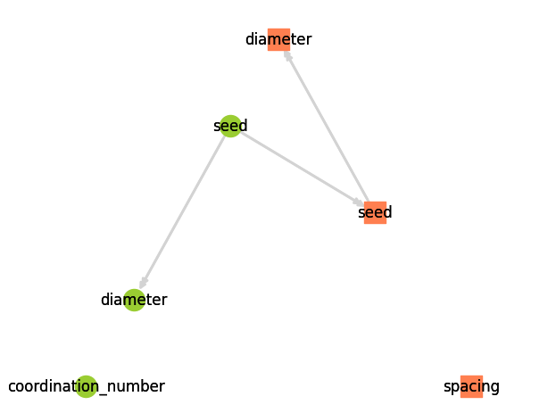
The green circles are pore properties and the orange squares are throat properties. We can also see that there are two models which are not dependent on anything else: 'throat.spacing' and 'pore.coordination_number'. These are added to all networks during generation but not run, hence their values do no show up when doing print(pn).
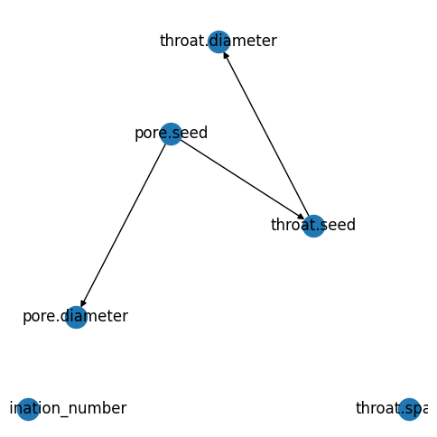
It is also possible to make your own plot if you wish, by retrieving the dependency graph then calling the networkx plotting function of your choice:
import networkx as nx
g = pn.models.dependency_graph()
fig, ax = plt.subplots(figsize=[5, 5])
nx.draw_networkx
nx.draw_planar(g, labels={k: k for k, v in g.nodes.items()}, ax=ax)