Getting Started#
It is relatively easy to get going with a quick simulation in OpenPNM. In fact the following code block produces a mercury intrusion simulation in just a few lines.
Creating a Cubic Network#
import openpnm as op
import numpy as np
import matplotlib.pyplot as plt
op.visualization.set_mpl_style()

Nx, Ny, Nz = 10, 10, 10
Lc = 1e-4
pn = op.network.Cubic([Nx, Ny, Nz], spacing=Lc)
pn.add_model_collection(op.models.collections.geometry.spheres_and_cylinders)
pn.regenerate_models()
print(pn)
══════════════════════════════════════════════════════════════════════════════
net : <openpnm.network.Cubic at 0x7f4793706df0>
――――――――――――――――――――――――――――――――――――――――――――――――――――――――――――――――――――――――――――――
  #  Properties                                                   Valid Values
――――――――――――――――――――――――――――――――――――――――――――――――――――――――――――――――――――――――――――――
  2  pore.coords                                                   1000 / 1000
  3  throat.conns                                                  2700 / 2700
  4  pore.coordination_number                                      1000 / 1000
  5  pore.max_size                                                 1000 / 1000
  6  throat.spacing                                                2700 / 2700
  7  pore.seed                                                     1000 / 1000
  8  pore.diameter                                                 1000 / 1000
  9  throat.max_size                                               2700 / 2700
 10  throat.diameter                                               2700 / 2700
 11  throat.cross_sectional_area                                   2700 / 2700
 12  throat.hydraulic_size_factors                                 2700 / 2700
 13  throat.diffusive_size_factors                                 2700 / 2700
 14  throat.lens_volume                                            2700 / 2700
 15  throat.length                                                 2700 / 2700
 16  throat.total_volume                                           2700 / 2700
 17  throat.volume                                                 2700 / 2700
 18  pore.volume                                                   1000 / 1000
――――――――――――――――――――――――――――――――――――――――――――――――――――――――――――――――――――――――――――――
  #  Labels                                                 Assigned Locations
――――――――――――――――――――――――――――――――――――――――――――――――――――――――――――――――――――――――――――――
  2  pore.xmin                                                             100
  3  pore.xmax                                                             100
  4  pore.ymin                                                             100
  5  pore.ymax                                                             100
  6  pore.zmin                                                             100
  7  pore.zmax                                                             100
  8  pore.surface                                                          488
  9  throat.surface                                                        972
 10  pore.left                                                             100
 11  pore.right                                                            100
 12  pore.front                                                            100
 13  pore.back                                                             100
 14  pore.bottom                                                           100
 15  pore.top                                                              100
――――――――――――――――――――――――――――――――――――――――――――――――――――――――――――――――――――――――――――――
Defining a Phase#
hg = op.phase.Mercury(network=pn)
hg.add_model(propname='throat.entry_pressure',
             model=op.models.physics.capillary_pressure.washburn)
hg.regenerate_models()
print(hg)
══════════════════════════════════════════════════════════════════════════════
phase_01 : <openpnm.phase.Mercury at 0x7f47e6b5c370>
――――――――――――――――――――――――――――――――――――――――――――――――――――――――――――――――――――――――――――――
  #  Properties                                                   Valid Values
――――――――――――――――――――――――――――――――――――――――――――――――――――――――――――――――――――――――――――――
  2  pore.temperature                                              1000 / 1000
  3  pore.pressure                                                 1000 / 1000
  4  throat.contact_angle                                          2700 / 2700
  5  pore.thermal_conductivity                                     1000 / 1000
  6  pore.surface_tension                                          1000 / 1000
  7  pore.viscosity                                                1000 / 1000
  8  pore.density                                                  1000 / 1000
  9  pore.molar_density                                            1000 / 1000
 10  throat.entry_pressure                                         2700 / 2700
――――――――――――――――――――――――――――――――――――――――――――――――――――――――――――――――――――――――――――――
  #  Labels                                                 Assigned Locations
――――――――――――――――――――――――――――――――――――――――――――――――――――――――――――――――――――――――――――――
  2  pore.all                                                             1000
  3  throat.all                                                           2700
――――――――――――――――――――――――――――――――――――――――――――――――――――――――――――――――――――――――――――――
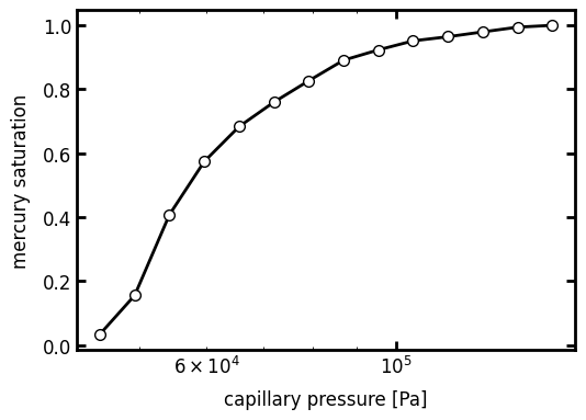
Performing a Drainage Simulation#
mip = op.algorithms.Drainage(network=pn, phase=hg)
mip.set_inlet_BC(pores=pn.pores(['left', 'right']))
mip.run(pressures=np.logspace(4, 6))
data = mip.pc_curve()
fig, ax = plt.subplots(figsize=(5.5, 4))
ax.semilogx(data.pc, data.snwp, 'k-o')
ax.set_xlabel('capillary pressure [Pa]')
ax.set_ylabel('mercury saturation');
Calculating Permeability Coefficient#
As another example, the permeability coefficient can be found as follows:
# Generate phase and physics
water = op.phase.Water(network=pn)
water.add_model(propname='throat.hydraulic_conductance',
                model=op.models.physics.hydraulic_conductance.generic_hydraulic)

# Create algorithm, set boundary conditions and run simulation
sf = op.algorithms.StokesFlow(network=pn, phase=water)
Pin, Pout = (200_000, 101_325)
sf.set_value_BC(pores=pn.pores('left'), values=Pin)
sf.set_value_BC(pores=pn.pores('right'), values=Pout)
sf.run()
The total flow rate into the domain through the boundary pores can be found
using sf.rate(pores=pn.pores('xmin')). The permeability coefficient
can be found by inserting known values into Darcy’s law as follows:
Q = sf.rate(pores=pn.pores('left'))
A = Ny*Nz*Lc**2
L = Nx*Lc
mu = water['pore.viscosity'].mean()
K = Q*mu*L/(A*(Pin-Pout))
print(K)
[8.28011364e-13]
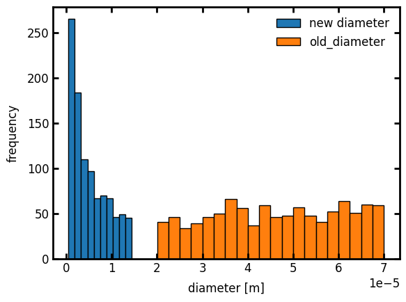
Adjusting Pore Size Distribution#
It’s also worth explaining how to adjust the pore size distribution of the network, so that the capillary curve and permeability coefficient can be changed to match known values. The geo object controls the geometric properties, and it possess models to calculate values on demand. Let’s change the pore size distribution to a Weibull distribution, but first let’s store the existing values in a dummy variable so we can compare later.
import openpnm.models.geometry as gmods

pn['pore.old_diameter'] = pn.pop('pore.diameter')
pn.add_model(propname='pore.diameter',
             model=gmods.pore_size.weibull,
             shape=0.5, loc=0, scale=1e-5)
Now you can use matplotlib. to get a quick glance at the histograms of the two distributions.
import matplotlib.pyplot as plt

fig, ax = plt.subplots(figsize=(6, 4.5))
ax.hist(pn['pore.diameter'], edgecolor='k', label='new diameter')
ax.hist(pn['pore.old_diameter'], edgecolor='k', label='old_diameter', bins=20)
ax.set_xlabel('diameter [m]')
ax.set_ylabel('frequency')
ax.legend();
More complex tasks are explained in the examples page.