Size Factors and Transport Conductance

Conductance in pore network models

Consider an arbitrary pore network model such as the one shown below:

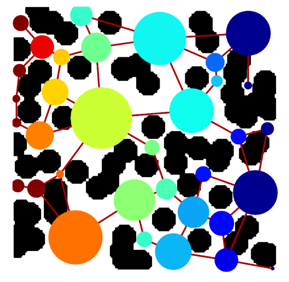
For simulating transport in this network, we need to know lots of parameters such as pore sizes, physical properties, etc, but ultimately it comes down to knowing the conductance of the “conduits” in the network. For example, consider simulating Fickian diffusion in a pore network model under steady state conditions. Writing a mass balance around an arbitrary pore \(i\), we have:

\[ \sum_k^{Nb^i} m_{ik} = \sum_k^{Nb^i} g_{ik} (c_i - c_k) = 0 \]

where \(Nb^i\) is the number of neighboring pores to pore \(i\), \(m_{ik}\) is the mass flow rate from pore \(i\) to pore \(k\), and \(g_{ik}\) is the overall conductance of the conduit containing pores \(i\) and \(k\), and the connecting throat \(ik\). In simple terms, it means that any mass that enters/exits pore \(i\) must balance such that the net rate is 0. Writing the mass balance for each pore, we get a linear system of \(N_p\) equations (where \(N_p\) is the total number of pores in the network), which can be solved for the pore concentrations using a linear solver.

Conductance of a single conduit

Consider a conduit in a pore network model, as shown by the following figure (we assumed spherical pores and cylindrical throats, but this is not necessary):

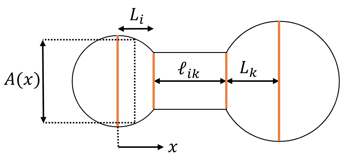
where L is length, A is the cross-sectional area, and the subscripts \(i\), \(k\), and \(ik\) denote pore \(i\), pore \(k\), and throat \(ik\). Now, consider the diffusional mass transfer between pore \(i\) and pore \(k\) with a mass flow rate of \(m_{ik}\), which can be described by the following equation:

(1)\[ m_{ik} = g_{ik} \cdot (c_i - c_k) \]

where \(g_{ik}\) is the overall conductance of the conduit \(ik\).

Note

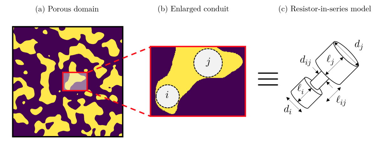
A conduit is the assembly of a throat and the two pores it connects. So, conduit \(ik\) is not the same as throat \(ik\)! The conduit \(ik\) begins at the center of pore \(i\) and ends at the center of pore \(k\).

The overall conductance is a function of the pore sizes, throat sizes, and physical properties of the fluid. Since elements of a conduit are connected in series, by electrical circuit analogy, the resistance (inverse of the conductance) of each element can be related to the overall resistance by the following equation:

\[ R_{ik} = R_i^p + R_k^p + R_{ik}^t \]

where the superscripts \(p\) and \(t\) denote pore and throat, respectively, and \(R_{ik}\) is the resistance of the entire conduit. The equation above can be rewritten in form of conductance as follows:

(2)\[ 1/g_{ik} = 1/g_i^p + 1/g_k^p + 1/g_{ik}^t \]

For simplicity, let’s assume that the shape of the pores and throats are cylindrical as shown in the figure below:

Based on this assumption, the diffusive conductance of each element can be expressed as (more on how to derive these equations comes later):

(3)\[ g_i^p = D \frac{\pi d_i^2/4}{\ell_i} \quad , \quad g_k^p = D \frac{\pi d_k^2/4}{\ell_k} \quad , \quad g_{ik}^t = D \frac{\pi d_{ik}^2/4}{\ell_{ik}} \]

Size factors vs. shape factors

In reality, however, pores/throats are not cylindrical, and the diffusive conductance needs to be corrected. This correction factor is called the shape factor in the network modeling literature, as defined by the following equation:

\[ SF = \frac{\text{actual conductance}}{\text{cylindrical conductance}} \]

Warning

We used to use shape factors in OpenPNM in the past, but for the sake of clarity, we removed them and introduced the concept of “size factor” instead. More on this later.

In OpenPNM, we used to follow this terminology, but because the shape factor depends on both geometrical and physical properties, we coined the term size factor, \(\mathcal{S}\) to decouple the geometric part of the conductance from its physical properties dependence, such that the diffusional mass flow rate becomes:

\[ m_{ik} = \mathcal{S} \cdot D \cdot (c_i - c_k) \]

where \(D\) is the diffusivity. In other words, the size factor is the geometric part of the conductance, and so the conductance can be defined in terms of the size factor as:

\[ g = \mathcal{S} \cdot D \]

for diffusive transport, and

\[ g = \mathcal{S} \cdot \frac{1}{\mu} \]

for fluid flow, where \(\mu\) is the viscosity.

Built-in size factor models in OpenPNM

OpenPNM has a number of built-in functions to calculate the size factor, which can be found under openpnm.models.geometry. Let’s inspect the available diffusive and hydraulic size factor models:

import openpnm as op
op.visualization.set_mpl_style()
op.Workspace().settings.loglevel = 50
diffusive_size_factors = op.models.geometry.diffusive_size_factors
print("\n".join(diffusive_size_factors._funcs.__all__))

spheres_and_cylinders
circles_and_rectangles
cones_and_cylinders
intersecting_cones
hybrid_cones_and_cylinders
trapezoids_and_rectangles
hybrid_trapezoids_and_rectangles
intersecting_trapezoids
pyramids_and_cuboids
intersecting_pyramids
hybrid_pyramids_and_cuboids
cubes_and_cuboids
squares_and_rectangles
intersecting_trapezoids
ncylinders_in_series

import openpnm as op
hydraulic_size_factors = op.models.geometry.hydraulic_size_factors
print("\n".join(hydraulic_size_factors._funcs.__all__))

spheres_and_cylinders
circles_and_rectangles
cones_and_cylinders
intersecting_cones
hybrid_cones_and_cylinders
trapezoids_and_rectangles
intersecting_trapezoids
hybrid_trapezoids_and_rectangles
pyramids_and_cuboids
intersecting_pyramids
hybrid_pyramids_and_cuboids
cubes_and_cuboids
squares_and_rectangles
ncylinders_in_series

Note

The diffusive size factor models can be used for any physics that involves molecular diffusion such as heat conduction, electron transport, etc, and therefore, it is not limited to the diffusive mass transport. The hydraulic size factor models, however, are only applicable to fluid flow algorithms such as StokesFlow.

Deriving the size factor for arbitrary-shaped pores and throats

In this section, we will derive the equation for the size factor for arbitrary-shaped pores and throats, then we will apply it to the case of cylindrical pores and throats to retrieve the equations we used in the previous section.

Consider the following conduit, which consists of pore \(i\), throat \(ik\), and pore \(k\):

Note that the choice of spheres and cylinders in the above figure is arbitrary and will not be taken into account in the derivation.

Diffusive size factor

From the Fick’s law of diffusion, the diffusive mass flow rate between pore \(i\) and pore \(k\) is given by (assuming that the transport begins at the center of pore \(i\) and ends at the center of pore \(k\)):

\[ m_{ik} = -D \cdot A(x) \cdot \frac{dc}{dx} \]

where \(A(x)\) is the cross-sectional area of the conduit at position \(x\), and \(dc/dx\) is the concentration gradient. Rearranging the equation above, we get:

\[ m_{ik} \cdot \frac{dx}{A(x)} = -D \cdot dc \]

Integrating the above equation over the entire conduit, we get:

\[ m_{ik} \int_{i \rightarrow k} \frac{dx}{A(x)} = -D \int_{i \rightarrow k} dc \]

Note that \(m_{ik}\) and \(D\) are not a function of \(x\), so they can be taken out of the integral. Since the conduit elements are connected in series, the above equation can be rewritten as:

\[ m_{ik} \Bigg[ \Big( \int \frac{dx}{A(x)} \Big)_{\text{pore }i} + \Big( \int \frac{dx}{A(x)} \Big)_{\text{throat }ik} + \Big( \int \frac{dx}{A(x)} \Big)_{\text{pore }k} \Bigg] = D \cdot (c_i - c_k) \]

and after rearranging, we get:

\[ m_{ik} = \Bigg[ \Big( \int \frac{dx}{A(x)} \Big)_{\text{pore }i} + \Big( \int \frac{dx}{A(x)} \Big)_{\text{throat }ik} + \Big( \int \frac{dx}{A(x)} \Big)_{\text{pore }k} \Bigg]^{-1} \cdot D \cdot (c_i - c_k) \]

By comparing the above equation with equations (1), and (2), we can get:

\[ \frac{1}{g_{ik}} = \frac{1}{g_i^p} + \frac{1}{g_{ik}^t} + \frac{1}{g_k^p} = \Bigg[ \Big( \int \frac{dx}{A(x)} \Big)_{\text{pore }i} + \Big( \int \frac{dx}{A(x)} \Big)_{\text{throat }ik} + \Big( \int \frac{dx}{A(x)} \Big)_{\text{pore }k} \Bigg] \cdot \frac{1}{D} \]

Combining the above equation with the definition of the diffusive size factor, \(g = \mathcal{S} \cdot D\), we get:

\[ \frac{1}{D} \cdot \frac{1}{\mathcal{S}_{ik}} = \frac{1}{D} \cdot \Bigg[ \frac{1}{\mathcal{S}_i^p} + \frac{1}{\mathcal{S}_{ik}^t} + \frac{1}{\mathcal{S}_k^p} \Bigg] = \Bigg[ \Big( \int \frac{dx}{A(x)} \Big)_{\text{pore }i} + \Big( \int \frac{dx}{A(x)} \Big)_{\text{throat }ik} + \Big( \int \frac{dx}{A(x)} \Big)_{\text{pore }k} \Bigg] \cdot \frac{1}{D} \]

Canceling the \(1/D\) terms, we can finally get the size factors for each conduit element:

\[ \mathcal{S}_{i}^p = \Big[ \int_{\ell_i} \frac{dx}{A_i(x)} \Big]^{-1} \quad , \quad \mathcal{S}_{ik}^t = \Big[ \int_{\ell_{ik}} \frac{dx}{A_{ik}(x)} \Big]^{-1} \quad , \quad \mathcal{S}_{k}^p = \Big[ \int_{\ell_k} \frac{dx}{A_k(x)} \Big]^{-1} \]

where \(A_i(x)\), \(A_k(x)\), and \(A_{ik}(x)\) are the cross-sectional areas of pores \(i\), \(k\), and throat \(ik\), respectively. Note that the above equations are valid for any arbitrary shape of the pores and throats.

As a test case, let’s consider cylindrical pores and throats. In this case, the cross-sectional area of the each element is given by:

(4)\[ A_i = \pi d_i^2/4 \quad , \quad A_k = \pi d_k^2/4 \quad , \quad A_{ik} = \pi d_{ik}^2/4 \]

where \(d_i\), \(d_k\), and \(d_{ik}\) are the diameters of pores \(i\), \(k\), and throat \(ik\), respectively. Substituting the above equations into the above equations, we get:

\[ \mathcal{S}_{i}^p = \frac{\pi d_i^2}{4 \cdot \ell_i} \quad , \quad \mathcal{S}_{ik}^t = \frac{\pi d_{ik}^2}{4 \cdot \ell_{ik}} \quad , \quad \mathcal{S}_{k}^p = \frac{\pi d_k^2}{4 \cdot \ell_k} \]

which matches what we declared earlier in equation (3).

Hydraulic size factor

For brevity, we will not go into the nitty-gritty details of the derivation of the hydraulic size factors. Instead, we will give you some pointers on where to start. The derivation of the hydraulic size factors is slightly more involved than that of the diffusive size factors. The main reason is that fluid flow equations need to satisfy two sets of boundary conditions, pressure drop along the domain (\(p_i\) and \(p_k\) at the two ends of the conduit), and no slip at the lateral boundaries (walls), whereas for diffusive transport, only the concentration boundary conditions need to be satisfied (\(c_i\) and \(c_k\) at the two ends of the conduit).

Assuming that the cross-section of the conduit is gradually changing, the pressure drop along the conduit can be approximated by the following equation [1]:

\[ -\frac{1}{Q} \frac{dp}{dx} = \mu \Big[ 16\pi^2 \cdot \frac{I_p^*}{A(x)^2} - \frac{2 \rho Q}{\mu} \cdot \frac{dA(x)/dx}{A(x)^3} \Big] \]

where \(Q\) is the volumetric flow rate, \(I_p^*\) is the specific polar moment of inertia [2] (don’t worry if you don’t know what this is, there are tables in the literature that you can use to look up the values for different shapes), \(A(x)\) is the cross-sectional area of the conduit, and \(\mu\) is the viscosity of the fluid. Rearranging and integrating the above equation, we get:

(5)\[ -\frac{1}{Q} \int dp = \mu \Big[ 16\pi^2 \int \frac{I_p^*}{A(x)} dx - \frac{2 \rho Q}{\mu} \cdot \int \frac{dA(x)/dx}{A(x)^3} dx \Big] \]

From calculus, we know that:

\[ \frac{dA(x)/dx}{A(x)^3} = - \frac{1}{2} \frac{d}{dx} \Big( \frac{1}{A(x)^2} \Big) \]

Substituting the above equation into equation (5), we get:

\[ \frac{p_i - p_j}{Q} = \mu \Big[ 16\pi^2 \int \frac{I_p^*}{A(x)} dx + \frac{\rho Q}{\mu} \cdot \int d \Big( \frac{1}{A(x)^2} \Big) \Big] \]

which can further be simplified to:

\[ \frac{p_i - p_j}{Q} = 16 \pi^2 \mu \int \frac{I_p^*}{A(x)^2} dx + \rho Q \cdot \Big( \frac{1}{A_k^2} - \frac{1}{A_i^2} \Big) \]

where the first term in the right-hand-side is the frictional loss, and the second term is the inertial loss. The frictional loss is a function of the conduit geometry, and the inertial loss is a function of the flow rate and the conduit geometry. The frictional loss is usually much larger than the inertial loss, so we can safely ignore the inertial loss to obtain:

(6)\[ \frac{p_i - p_j}{Q} = 16 \pi^2 \mu \int \frac{I_p^*}{A(x)^2} dx \]

Similar to the diffusive transport, the hydraulic conductance is defined as the ratio of the flow rate to the pressure drop as follows:

(7)\[ Q = g_{ik} \cdot (p_i - p_k) \]

where \(g_{ik}\) is the hydraulic conductance (we use the same notation as the diffusive conductance to keep it simple in this notebook). Expanding the integral over the conduit on each element (pores \(i\) and \(k\), and throat \(ik\)), and by comparing equations (6) and (7), we get:

\[ \frac{1}{g_{ik}} = \frac{1}{g_i^p} + \frac{1}{g_{ik}^t} + \frac{1}{g_k^p} = 16 \pi^2 \mu \Bigg[ \Bigg( \int \frac{I_p^*}{A_i(x)^2} dx \Bigg)_{\text{pore } i} + \Bigg( \int \frac{I_p^*}{A_{ik}(x)^2} dx \Bigg)_{\text{throat }ik} + \Bigg( \int \frac{I_p^*}{A_k(x)^2} dx \Bigg)_{\text{pore } k} \Bigg] \]

Combining the above equation with the definition of the hydraulic size factor, \(g = \mathcal{S} / \mu\), we get:

\[ \frac{\mu}{\mathcal{S}_{ik}} = \mu \cdot \Bigg[ \frac{1}{\mathcal{S}_i^p} + \frac{1}{\mathcal{S}_{ik}^t} + \frac{1}{\mathcal{S}_k^p} \Bigg] = 16 \pi^2 \mu \Bigg[ \Bigg( \int \frac{I_p^*}{A_i(x)^2} dx \Bigg)_{\text{pore } i} + \Bigg( \int \frac{I_p^*}{A_{ik}(x)^2} dx \Bigg)_{\text{throat }ik} + \Bigg( \int \frac{I_p^*}{A_k(x)^2} dx \Bigg)_{\text{pore } k} \Bigg] \]

from which, we can obtain the hydraulic size factor for each conduit element as follows:

(8)\[ \mathcal{S}_{i}^p = \Big[ 16 \pi^2 \int_{\ell_i} \frac{I_p^*}{A_i(x)^2} dx \Big]^{-1} \quad , \quad \mathcal{S}_{ik}^t = \Big[ 16 \pi^2 \int_{\ell_{ik}} \frac{I_p^*}{A_{ik}(x)^2} dx \Big]^{-1} \quad , \quad \mathcal{S}_{k}^p = \Big[ 16 \pi^2 \int_{\ell_k} \frac{I_p^*}{A_k(x)^2} dx \Big]^{-1} \]

As a test case, consider cylidnrical pores and throats. The specific polar moment of inertia for a cylinder is:

\[ I_p^* = \frac{1}{4 \pi} \]

Substituting the above equation and the cross-sectional areas from equation (4) into equation (8), we get:

\[ \mathcal{S}_{i}^p = \frac{\pi d_i^4}{128} \quad , \quad \mathcal{S}_{ik}^t = \frac{\pi d_{ik}^4}{128} \quad , \quad \mathcal{S}_{k}^p = \frac{\pi d_k^4}{128} \]

To verify the above results, we can inspect the Hagen-Poiseuille equation for a cylindrical conduit [3]:

\[ \Delta p = \frac{8 \pi \mu \ell Q}{A^2} \Rightarrow \frac{Q}{\Delta p} = \frac{A^2}{8 \pi \mu \ell} = \frac{\pi d^4}{128 \mu \ell} \]

Since the hydraulic size factor is defined as \(g / \mu\), and the hydraulic conductance is defined as \(Q / \Delta p\), we can derive the following relationship for the hydraulic size factor based on the Hagen-Poiseuille equation:

\[ \mathcal{S} = \frac{\pi d^4}{128 \ell} \]

which matches our derivation.

Conduit vs. element size factor

So far, we have derived individual equations for the size factor of each conduit element as well the entire conduit (based on resistors in series model). Note that eventually, only the size factor of the entire conduit is used by the algorithms, although as we discussed, it is directly calculated from the size factors of the individual elements.

Almost all of the built-in size factor models in OpenPNM return an Nt by 3 array, where Nt is the number of conduits (same as the number of throats!). The first column is the size factor of the pore on the left side of the conduit, the second column is the size factor of the throat, and the third column is the size factor of the pore on the right side of the conduit.

However, we do have one model (at the time of writing this notebook) that uses a machine learning method [4] to predict the diffusive size factor of the entire conduit directly from a voxel image of the porous medium. For this reason, it only returns an Nt by 1 vector. Our built-in conductance models (which take in the size factor and physical properties as input and return the conductance) are designed to work with both types of size factor models.

---

[1]

Akbari, M., D. Sinton, and M. Bahrami. “Viscous flow in variable cross-section microchannels of arbitrary shapes.” International Journal of Heat and Mass Transfer 54.17-18 (2011): 3970-3978.

[2]

Bahrami, Majid, M. Michael Yovanovich, and J. Richard Culham. “A novel solution for pressure drop in singly connected microchannels of arbitrary cross-section.” International Journal of Heat and Mass Transfer 50.13-14 (2007): 2492-2502.

[3]

https://en.wikipedia.org/wiki/Hagen%E2%80%93Poiseuille_equation

[4]

Misaghian, Niloo, et al. “Prediction of diffusional conductance in extracted pore network models using convolutional neural networks.” Computers & Geosciences 162 (2022): 105086.